Angular velocity from Quaternions

We all know we can obtain a pose represented as a quaternion by simply integrating the measured angular velocities. You got these velocities from a gyroscope, for example. It is as easy as summing them up over time.

Of course, the mathematical background is a bit more complicated but that is the principle. And the other way around is possible too. From the different poses we could get the angular velocities between them (given a time period.)

I just cannot understand why I havent found an easy implementation of this in the wild west we know as internet. It is, at least for me, one of the most useful data one can get from a set of orientations.

I’m gonna try to explain how we can easily obtain it, including some real life examples.

Quaternions

First, let’s define our Quaternion representation according to Hamilton’s notation:

$$\mathbf{q} = q_w + q_x\mathbb{i} + q_y\mathbb{j} + q_z\mathbb{k} = \begin{bmatrix}q_w \\ q_x \\ q_y \\ q_z\end{bmatrix} = \begin{pmatrix}q_w \\ \mathbf{q_v}\end{pmatrix}$$

where \(q_w\) is the scalar part, and \(\mathbf{q_v}\) is the vector part of the quaternion.

This quaternion can represent two things when normalized (normalized means \(\|\mathbf{q}\|=1\)):

• It is an orientation with respect to the global frame, but represented with 4 dimensions.
• It is a rotation operation, which is basically moving a particle around an axis at a certain angle.

For this case we use the former intepretation. It represents an orientation.

It is difficult to visualize this, but an easy conversion in 3D is the well known matrix:

$$\mathbf{R}(\mathbf{q}) =\begin{bmatrix}1 - 2(q_y^2 + q_z^2) & 2(q_xq_y - q_wq_z) & 2(q_xq_z + q_wq_y) \\2(q_xq_y + q_wq_z) & 1 - 2(q_x^2 + q_z^2) & 2(q_yq_z - q_wq_x) \\2(q_xq_z - q_wq_y) & 2(q_wq_x + q_yq_z) & 1 - 2(q_x^2 + q_y^2)\end{bmatrix}$$

where \(\mathbf{R}\) is the \(3\times 3\) Direction Cosine Matrix used to represent the same orientation, but in three dimensions.

Quaternion Derivative

Angular rates, \(\boldsymbol\omega(t)=\begin{bmatrix}\omega_x&\omega_y&\omega_z\end{bmatrix}^T\), in rad/s, are measured by gyroscopes at any time \(t\) in the local sensor frame.

It is after a rotation change \(\Delta\mathbf{q}\) during \(\Delta t\) seconds that we arrive to a new orientation \(\mathbf{q} (t+\Delta t)\). The parameter \(\Delta t\) is the “time step” or “step size”, which is the time passed between each measurement.

The first derivative of the orientation, \(\dot{\mathbf{q}}\), is what we try to measure with the gyroscopes. However, the derivative of the quaternion is in 4 dimensions:

$$\begin{array}{rcl}\dot{\mathbf{q}} &=& \underset{\Delta t\to 0}{\mathrm{lim}} \frac{\mathbf{q}(t+\Delta t)-\mathbf{q}(t)}{\Delta t} \\ \\ &=& \frac{1}{2}\boldsymbol\Omega(\boldsymbol\omega)\mathbf{q}\end{array}$$

where \(\boldsymbol\Omega(\boldsymbol\omega)\) is the Omega operator:

$$\boldsymbol\Omega(\boldsymbol\omega) = \begin{bmatrix}0 & -\boldsymbol\omega^T \\ \boldsymbol\omega & \lfloor\boldsymbol\omega\rfloor_\times\end{bmatrix} = \begin{bmatrix}0 & -\omega_x & -\omega_y & -\omega_z \\ \omega_x & 0 & \omega_z & -\omega_y \\ \omega_y & -\omega_z & 0 & \omega_x \\ \omega_z & \omega_y & -\omega_x & 0\end{bmatrix}$$

For a more detailed description of this derivative you can check the Angular Rate Estimator in Python’s Package AHRS.

Quaternion Integration

What we need, however, is the three-dimensional angular velocity \(\boldsymbol{\omega}\) relating the two quaternions \(\mathbf{q}(t)\) and \(\mathbf{q}(t+\Delta t)\).

This can be quickly achieved by analyzing the Integral between these Quaternions.

Assuming the angular rate is constant over the period \([t, t+\Delta t]\), meaning the angular acceleration is zero (\(\dot{\boldsymbol{\omega}}=\mathbf{0}\)), we can build a Taylor series around the time \(t\):

$$\mathbf{q}(t+\Delta t) = \Bigg[\mathbf{I}_4 + \frac{1}{2}\boldsymbol\Omega(\boldsymbol\omega)\Delta t + \frac{1}{2!}\Big(\frac{1}{2}\boldsymbol\Omega(\boldsymbol\omega)\Delta t\Big)^2 + \frac{1}{3!}\Big(\frac{1}{2}\boldsymbol\Omega(\boldsymbol\omega)\Delta t\Big)^3 + \cdots\Bigg]\mathbf{q}(t)$$

Notice the series has the known form of the matrix exponential:

$$e^{\mathbf{X}} = \sum_{k=0}^\infty \frac{1}{k!} \mathbf{X}^k$$

Now we have a term based on \(\boldsymbol{\omega}\) relating both quaternions.

$$\begin{array}{rcl}\mathbf{q}(t+\Delta t) &=& e^{\frac{\Delta t}{2}\boldsymbol\Omega(\boldsymbol\omega)} \mathbf{q}(t) \\ &=& \Bigg[\sum_{k=0}^\infty \frac{1}{k!} \Big(\frac{\Delta t}{2}\boldsymbol\Omega(\boldsymbol\omega)\Big)^k\Bigg] \mathbf{q}(t) \end{array}$$

The more terms we allow, the more precise will be the approximation. But this becomes cumbersome for real applications. In most cases, nevertheless, the approximation after \(k=1\) is already good enough, and the equation is reduced to two terms only.

$$\begin{array}{rcl}\mathbf{q}(t+\Delta t) &=& \Bigg[\mathbf{I}_4 + \frac{1}{2}\boldsymbol\Omega(\boldsymbol\omega)\Delta t\Bigg]\mathbf{q}(t) \\ \begin{bmatrix}q_w(t+\Delta t) \\ q_x(t+\Delta t) \\ q_y(t+\Delta t) \\ q_z(t+\Delta t) \end{bmatrix} &=& \frac{\Delta t}{2} \begin{bmatrix}\frac{2}{\Delta t} & -\omega_x & -\omega_y & -\omega_z \\ \omega_x & \frac{2}{\Delta t} & \omega_z & -\omega_y \\ \omega_y & -\omega_z & \frac{2}{\Delta t} & \omega_x \\ \omega_z & \omega_y & -\omega_x & \frac{2}{\Delta t}\end{bmatrix} \begin{bmatrix}q_w(t) \\ q_x(t) \\ q_y(t) \\ q_z(t) \end{bmatrix}\end{array}$$

This linear operation rotates \(\mathbf{q}(t)\) to \(\mathbf{q}(t+\Delta t)\).

Thanks to Houcine Turki for its valuable correction of this equation.

The Angular Velocities

After a closer look we can identify our precious angular velocity at the first column of the linear operator. For me the most logical way is, then, to clear for \([\mathbf{I}_4 + \boldsymbol\Omega(\boldsymbol\omega) ]\)

Following the operations above we get:

$$\begin{bmatrix}q_w(t+\Delta t) \\ q_x(t+\Delta t) \\ q_y(t+\Delta t) \\ q_z(t+\Delta t) \end{bmatrix} = \frac{\Delta t}{2}\begin{bmatrix}-\omega_x q_x(t) - \omega_y q_y(t) - \omega_z q_z(t) + q_w(t) \\ \omega_x q_w(t) - \omega_y q_z(t) + \omega_z q_y(t) + q_x(t)\\ \omega_x q_z(t) + \omega_y q_w(t) - \omega_z q_x(t) + q_y(t)\\- \omega_x q_y(t) + \omega_y q_x(t) + \omega_z q_w(t) + q_z(t)\end{bmatrix}$$

Clearing for \([\mathbf{I}_4 + \boldsymbol\Omega(\boldsymbol\omega) ]\):

$$\begin{bmatrix}1 & -\omega_x & -\omega_y & -\omega_z \\ \omega_x & 1 & \omega_z & -\omega_y \\ \omega_y & -\omega_z & 1 & \omega_x \\ \omega_z & \omega_y & -\omega_x & 1\end{bmatrix} = \frac{2}{\Delta t} \begin{bmatrix} q_w(t) q_w(t+\Delta t) + q_x(t) q_x(t+\Delta t) + q_y(t) q_y(t+\Delta t) + q_z(t) q_z(t+\Delta t) & - q_w(t) q_x(t+\Delta t) + q_x(t) q_w(t+\Delta t) + q_y(t) q_z(t+\Delta t) - q_z(t) q_y(t+\Delta t) & - q_w(t) q_y(t+\Delta t) - q_x(t) q_z(t+\Delta t) + q_y(t) q_w(t+\Delta t) + q_z(t) q_x(t+\Delta t) & - q_w(t) q_z(t+\Delta t) + q_x(t) q_y(t+\Delta t) - q_y(t) q_x(t+\Delta t) + q_z(t) q_w(t+\Delta t) \\ q_w(t) q_x(t+\Delta t) - q_x(t) q_w(t+\Delta t) - q_y(t) q_z(t+\Delta t) + q_z(t) q_y(t+\Delta t) & q_w(t) q_w(t+\Delta t) + q_x(t) q_x(t+\Delta t) + q_y(t) q_y(t+\Delta t) + q_z(t) q_z(t+\Delta t) & q_w(t) q_z(t+\Delta t) - q_x(t) q_y(t+\Delta t) + q_y(t) q_x(t+\Delta t) - q_z(t) q_w(t+\Delta t) & - q_w(t) q_y(t+\Delta t) - q_x(t) q_z(t+\Delta t) + q_y(t) q_w(t+\Delta t) + q_z(t) q_x(t+\Delta t) \\ q_w(t) q_y(t+\Delta t) + q_x(t) q_z(t+\Delta t) - q_y(t) q_w(t+\Delta t) - q_z(t) q_x(t+\Delta t) & - q_w(t) q_z(t+\Delta t) + q_x(t) q_y(t+\Delta t) - q_y(t) q_x(t+\Delta t) + q_z(t) q_w(t+\Delta t) & q_w(t) q_w(t+\Delta t) + q_x(t) q_x(t+\Delta t) + q_y(t) q_y(t+\Delta t) + q_z(t) q_z(t+\Delta t) & q_w(t) q_x(t+\Delta t) - q_x(t) q_w(t+\Delta t) - q_y(t) q_z(t+\Delta t) + q_z(t) q_y(t+\Delta t) \\ q_w(t) q_z(t+\Delta t) - q_x(t) q_y(t+\Delta t) + q_y(t) q_x(t+\Delta t) - q_z(t) q_w(t+\Delta t) & q_w(t) q_y(t+\Delta t) + q_x(t) q_z(t+\Delta t) - q_y(t) q_w(t+\Delta t) - q_z(t) q_x(t+\Delta t) & - q_w(t) q_x(t+\Delta t) + q_x(t) q_w(t+\Delta t) + q_y(t) q_z(t+\Delta t) - q_z(t) q_y(t+\Delta t) & q_w(t) q_w(t+\Delta t) + q_x(t) q_x(t+\Delta t) + q_y(t) q_y(t+\Delta t) + q_z(t) q_z(t+\Delta t)\end{bmatrix}$$

We return to the \(4\times 4\) linear operator from above, but this time is defined entirely by the time step and quaternions \(\mathbf{q}(t)\) and \(\mathbf{q}(t+\Delta t)\). As noted before, we now identify the angular velocities from the first column:

$$\begin{array}{rcl}\omega_x &=& \frac{2}{\Delta t}\Big(q_w(t) q_x(t+\Delta t) - q_x(t) q_w(t+\Delta t) - q_y(t) q_z(t+\Delta t) + q_z(t) q_y(t+\Delta t)\Big) \\ \\ \omega_y &=& \frac{2}{\Delta t}\Big(q_w(t) q_y(t+\Delta t) + q_x(t) q_z(t+\Delta t) - q_y(t) q_w(t+\Delta t) - q_z(t) q_x(t+\Delta t)\Big) \\ \\ \omega_z &=& \frac{2}{\Delta t}\Big(q_w(t) q_z(t+\Delta t) - q_x(t) q_y(t+\Delta t) + q_y(t) q_x(t+\Delta t) - q_z(t) q_w(t+\Delta t)\Big)\end{array}$$

And that’s pretty much it. You can obtain the angular velocites between two quaternions given the time spent between them with the equations above.

Python implementation

A simple Python function of this computation is:

import numpy as np
def angular_velocities(q1, q2, dt):
    return (2 / dt) * np.array([
        q1[0]*q2[1] - q1[1]*q2[0] - q1[2]*q2[3] + q1[3]*q2[2],
        q1[0]*q2[2] + q1[1]*q2[3] - q1[2]*q2[0] - q1[3]*q2[1],
        q1[0]*q2[3] - q1[1]*q2[2] + q1[2]*q2[1] - q1[3]*q2[0]])

This takes the first quaternion \(\mathbf{q}(t)\), the second quaternion \(\mathbf{q}(t+\Delta t)\), and the time step \(\Delta t\) to compute the instantaneous angular velocity \(\boldsymbol\omega(t)=\begin{bmatrix}\omega_x&\omega_y&\omega_z\end{bmatrix}^T\).

Example

To show an example, I use the RepoIMU dataset, which includes calibrated measurements of the gyroscopes and synchronized orientations (as quaternions) measured with optical devices.

Here we see the poses as quaternions measured by the optical VICON system:

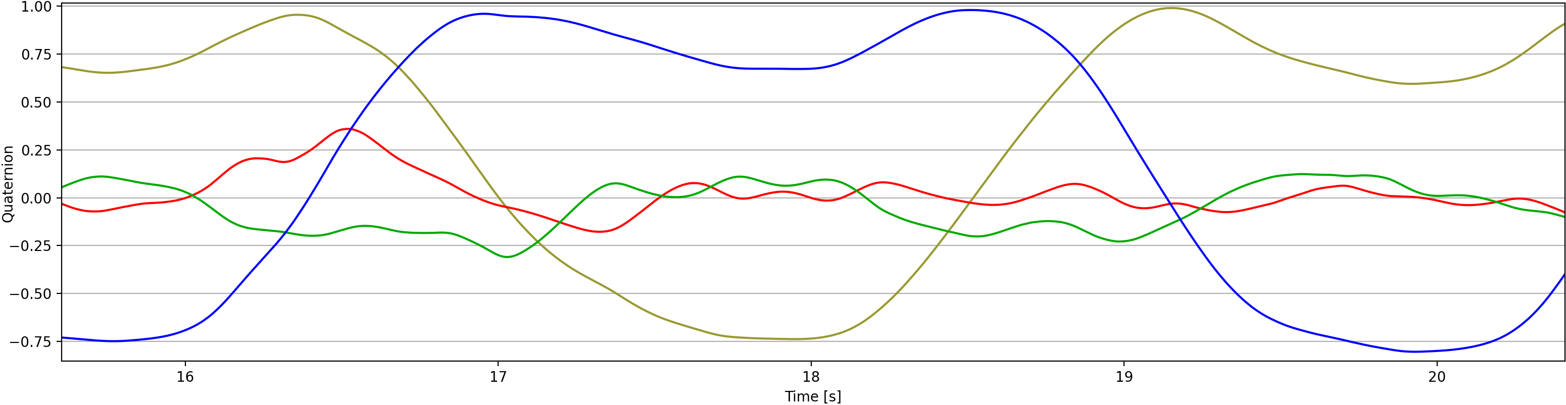
Using our function defined above, we obtain the angular velocities between them with a simple loop. Notice we will obtain \(N-1\) angular velocites from \(N\) quaternions:

array = np.loadtxt(data_file, dtype=float, delimiter=';', skiprows=2)
times = array[:, 0]
quaternions = array[:, 1:5]
gyroscopes = array[:, 8:11]
angvel = np.zeros_like(gyroscopes)
for i in range(1, len(angvel)):
    dt = times[i] - times[i-1]
    angvel[i] = angular_velocities(quaternions[i-1], quaternions[i], dt)

In this case, if we obtain angular velocites from the measured quaternions, they should match the measured ones from the gyroscopes.

Let’s plot the same times from above with the measured quaternions (using gyroscopes), and the estimated ones (with our function) in bold, side to side:

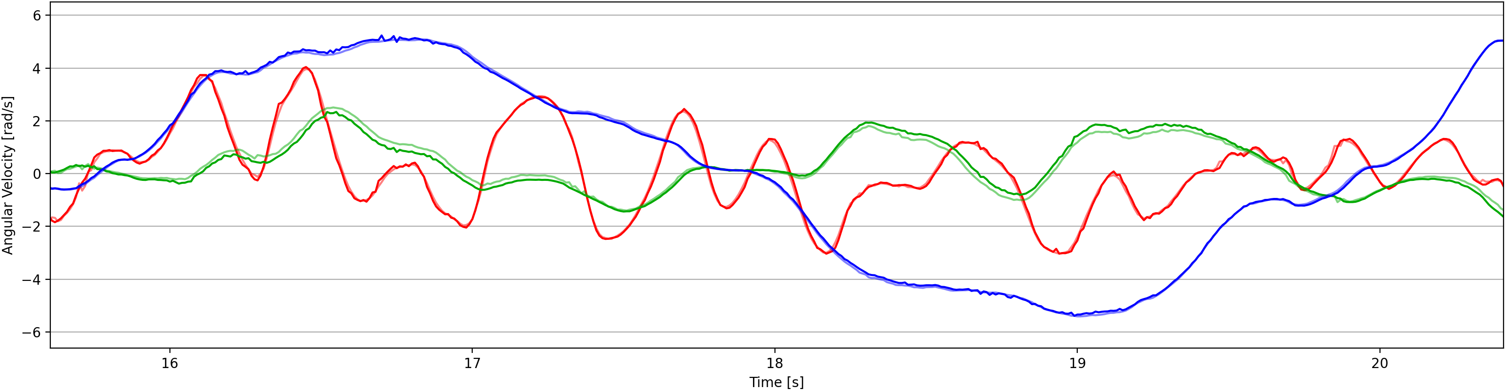
Their difference is very minimal. These differences between measured and estimated angular velocites can be due to noisy sensors, biases, and loss of accuracy in its linearization.

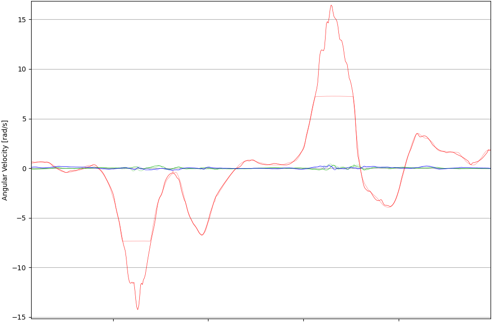
But in some cases we can even obtain angular velocites so big that the gyroscopes cannot measure (gyroscopes have a maximum range), but the optical systems could measure:

AHRS Implementation

The estimation of the angular velocity using this method has been added to the newest version of Python’s AHRS Package. Such implementation is vectorized to improve its performance.

It assumes, nevertheless, that the time step is constant throughout the recording, and we give it as a single float. With AHRS, we simply do:

import ahrs
Q = ahrs.QuaternionArray(quaternions)
ang_vels = Q.angular_velocities(np.diff(times).mean())

Opportunities for Improvement

We can increase the accuracy by increasing the order in the Taylor approximation, and clearing again for the linear operator.

In my case, however, it already satisfies the basic need of obtaining a “good enough” approximation for \(\boldsymbol\omega(t)\).