Kalman Filter. A painless approach
Posted

Any decent technological project will use this robust method for the final estimation of the position of any intelligent system. The format of the given information can be, fortunately, represented as a Gaussian state.
Thanks to this property, it is possible to use Gaussian filters (KF is one of them), in order to improve the final estimation.
Gaussian modelling estimations are going to be carried in this explanation, so it is preferable to have this mathematical background (a simple understanding is enough) in order to follow the presented technique.
The estimation problem
Let us go straight to the problem with an example. Suppose we have a robot moving freely in a 2D Euclidean space (Cartesian coordinates), and we want to track its real position every time.

There are several methods to do so and their mix in an adequate way is the secret to the best estimation. The first way is to mathematically estimate the position with simple physical models. Here classical Physics is our big allied and we can roughly use accelerations, velocities, etc.
At the beginning (time is equal to zero), our robot is set to be in the origin and, thanks to our mathematical model, we know that in the next second it will change its position to somewhere further in the field.
The position can be represented as a two-dimensional vector that represents the position along the X- and Y-axis, respectively. This vector is known as the “state vector”, because it contains the information of the robot in its current state.
Because this vector also represents an estimation, we will write it with a small “hat” as $$\mathbf{\hat{x}}$$. It is read as “x hat” and just means that this vector is an estimation (not precisely the true value).
$$\mathbf{\hat{x}} = \begin{pmatrix} \hat{x} \ \hat{y} \end{pmatrix}$$
For compliance with standard notation in Engineering, we denote time with $$t$$ and the set of sampled states as $$t_k={t_0,t_1,\cdots t_n }\in\mathbb{R}^{n+1}$$ where $$n$$ is positive semi-definite (greater than or equal to zero).
This funny notation simply means that the index of the time begins in zero and increases positively until $$n+1$$ values.
Under this convention, if we set the beginning at zero and estimate 5 more states, the time set is represented as $$t_k = {t_0, t_1, t_2, t_3, t_4, t_5}$$. Here $$n$$ is equal to 5, and the number of states is 6 (because we include $$t_0$$).
After a mathematical calculation (with classical physics), the robot is estimated to be in a specified new location:

However, due to a plethora of external forces and effects, the estimation of its position cannot be entirely deterministic and is prone to errors.
The robot can be in the estimated position our somewhere around it, because the mentioned effects can drive it up, down, left, right, the mix of them, or even stay in the same place. It could be anywhere around this original estimation.

This leads to the concept of variance. The variance represents how far a bunch of values is spread out.
| Large variance | Small variance |
|---|---|
 |
 |
For our robot a higher variance means that its real position can be far from the original estimation, while a smaller variance means that it can be closer to the estimated position.
Too many drawings of a robot. Let us use the “particle representation”. From now on, the mean position of the robot will be represented with a dot, and its variance with an ellipse around it. This ellipse is the most probable area, where the robot can be located.

As seen, using only mathematical models is not enough to locate the real position of our robot. But now, we are able to equip the robot with sensors.
These sensors can be integrated on the wheels (wheel encoders) and will measure the translation of our robot along X- and Y-axis.
The exclusive use of sensors for position estimation and tracking is known as Odometry. Simple Odometry is widely used in basic implementations of tracking and is enough for easy examples, but not for real cases, like the estimations of our robot.
Using the information of the wheel encoders in the robot, we can measure how far the robot moved after one timestamp. This will allow us to calculate its position and store it in a vector $$\mathbf{z}$$ commonly known as the measurement vector.
$$\mathbf{z} = \begin{pmatrix}\mathbf{z}_x \ \mathbf{z}_y\end{pmatrix}$$
But here we find the same flaw as the pure mathematical model: variance. No sensor is perfect and all of them include always some noise that disturbs the real measurement. Luckily this noise is a Gaussian noise and can be modelled as:
$$\mathbf{z}=\mathbf{z}_{real} +\mathbf{v}$$
This $$\mathbf{v}$$ is a perturbation within the variance of the sensor that changes the measurement around the real value and it is assumed to be independent to any other parameter. Visually, the position estimation based merely on sensors can be seen as:

The dot in the centre is the estimated position given by the sensors (mean) and the ellipse around is the variance of the sensor (the real position is most probably anywhere inside it). The better the sensor, the smaller the variance.
Both estimations, through Odometry and classical Physics, are not perfect and present some variance. This, of course, means that the computations are never going to be perfect. That same property of variance, however, is used to estimate a better position if we apply basic concepts of a mixture of Gaussians (MoG).
The definitions of MoG are not in the scope of this article, but the Gaussian properties are used to build the famous Kalman Filter.
The intuition behind KF
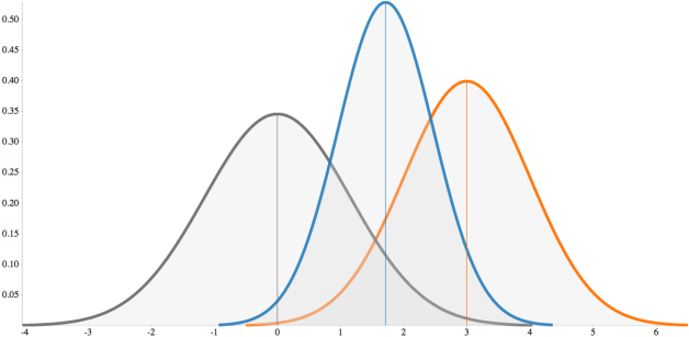
The mixture of two Gaussian distributions will give another Gaussian distribution. Thanks to this property, we are able to construct as many distributions as desired, provided that we are always using the proper ones.
The distributions used to build the “mixed distribution” are called priors, while the resulting new distribution is called a posterior.
This yields to the definition of Covariance, which is a measure of how much two random variables change together. If two distributions are the same (almost impossible in real life) then the covariance is equal to the variance of any distribution.
The variables show similar behaviour when the covariance is positive. Random variables whose covariance is zero are called uncorrelated.
For a further analysis on the development of these models, please refer to any documentation about Bayesian Inference. Here the understanding of the above definitions is enough.
The awesomeness of the KF lies in its capacity to take the values of the estimations (from Odometry and Models), their covariance, and compute a new Gaussian distribution, based only on the priors. This means, the KF takes calculations and measurements (as gaussian distributions) and estimates a better approximation to the real value, also as gaussian.
So, back to our robot example. We begin in the origin (set to zero), we predict its position (a priori state) and make a measurement with our sensors (observation). This will give us two different mean values (centres) and their corresponding variances (ellipses).
What KF will do is take these gaussian representations, mix them and estimate a new posterior with higher accuracy than the priors. This posterior is the final estimation of the position.
Obviously, a smaller covariance (ellipse) means a more accurate estimation. The best part is that the posterior has always a smaller covariance than any of the two priors. That is why it is always more accurate.
If the estimations are gaussian, the probability of their perturbations can be modelled as:
$$p(w)\sim \mathcal{N}(0,\mathbf{Q})$$
$$p(v)\sim \mathcal{N}(0,\mathbf{R})$$
The random variables $$w$$ and $$v$$ represent the process noise and measurement noise, respectively. They are assumed to be independent of each other, and with normal probability distribution.
The integration of noises $$w$$ and $$v$$ into their corresponding models can be defined as:
$$x_{calculated}=x_{real} + w$$
$$z_{calculated}=z_{real} + v$$
In practice, the process noise covariance $$\mathbf{Q}$$ and measurement noise covariance $$\mathbf{R}$$ matrices might change, but here are assumed to be constant. These noise covariance matrices define the shape of the ellipses in the example of our robot.
The precise way the KF will estimate the a posteriori state is based in the blending factor, also known as Kalman gain, represented only with a $$\mathbf{K}$$. The Kalman gain minimizes the a posteriori error covariance, by fusing the covariances into a new one based on their “heaviness”.
$$\mathbf{K} = \frac{\textrm{Predicted Covariance}}{\textrm{Predicted Covariance} + \textrm{Measurement Covariance}}$$
A simple way of thinking about $$\mathbf{K}$$ is: as the Measurement Covariance $$\mathbf{R}$$ approaches to zero (towards noiseless sensors), the actual measurement $$\mathbf{z}$$ should be trusted more and more, while the Predicted measurement is trusted less and less.
On the other hand, as the a priori estimate error covariance approaches to zero (towards perfect calculations), the actual measurement $$\mathbf{z}$$ is trusted less and less, while the predicted measurement is trusted more and more.
In simpler words: whenever $$\mathbf{K}$$ is equal to zero trust the calculations, and when $$\mathbf{K}$$ is equal to one trust the sensor.
The comparison between both quantities is, however, not always a simple one-to-one relation, where the calculations match perfectly with the measurements. Sometimes, in order to estimate positions, related operations in accelerations and velocities must be carried out, and these values are also stored and handled in the same vector. The sensors, in the other hand, give only one magnitude for the physical event they are measuring.
In order to match the corresponding values from calculations and measurements, it is necessary to use an Observation Matrix $$\mathbf{H}$$ that will pair the corresponding values. So, for example, if in our robot we use accelerometers instead of wheel encoders, we would need to estimate the position from the acceleration and then compare it with the mathematical estimations of our model. But for that we have to select only the part we are interested in: the position.
Assuming that the state vector has three elements: estimated position $$(\hat{x}{p})$$, estimated velocity $$(\hat{x}{v})$$ and estimated acceleration $$(\hat{x}_{a})$$, the only value that we can compare with a sensor is the estimated acceleration (if we only use accelerometers, of course). So we extract it from the state vector as:
$$\hat{x}{a} = \underbrace{\begin{pmatrix} 0 & 0 & 1 \end{pmatrix}}{\mathbf{H}} \underbrace{\begin{pmatrix} \hat{x}{p} \ \hat{x}{v} \ \hat{x}{a} \end{pmatrix}}{\mathbf{\hat{x}}}$$
Here we see that we just multiply the state vector $$\mathbf{\hat{x}}$$ with the $$3\times 1$$ observation matrix H to obtain only the last element $$\hat{x}_{a}$$ of the state vector. Why? To directly compare it against the measurement from the sensor:
$$\mathbf{r} = \mathbf{z} - \mathbf{H\hat{x}}$$
The resulting value $$\mathbf{r}$$ is the difference between the estimated measurement $$\mathbf{H\hat{x}}$$ and the actual measurement from the sensors $$\mathbf{z}$$. This vector $$\mathbf{r}$$ is called Innovation, Measurement Residual or just Residual, and its length is determined by the number of elements to be compared.
Adding a position sensor (like the wheel encoders) would give us the magnitude of the translation. This value can be also added to the measurement vector $$\mathbf{z}$$:
$$\mathbf{z} = \begin{pmatrix} z_\textrm{position} \ z_\textrm{acceleration} \end{pmatrix}$$
It yields an innovation vector $$\mathbf{r}$$:
$$\mathbf{z} = \begin{pmatrix} z_\textrm{position} \ z_\textrm{acceleration} \end{pmatrix} - \underbrace{\begin{pmatrix} 1 & 0 & 0 \ 0 & 0 & 1 \end{pmatrix}}{\mathbf{H}} \underbrace{\begin{pmatrix} \hat{x}{p} \ \hat{x}{v} \ \hat{x}{a} \end{pmatrix}}{\mathbf{\hat{x}}} = \begin{pmatrix} z\textrm{position} - \hat{x}{p} \ z\textrm{acceleration} - \hat{x}_{a} \end{pmatrix}$$
$$\mathbf{H}$$ decides who fights whom, $$\mathbf{r}$$ checks who punches stronger, and $$\mathbf{K}$$ decides who won.
Once we have the difference of the estimated and measured positions, we have to know how much we trust this difference, so we can add it to our previous estimation.
Which element tells us the confidence of our estimations? The Kalman gain! So, we just update the state with the weighted difference:
$$\mathbf{\hat{x}}\textrm{posterior} = \mathbf{\hat{x}}\textrm{prior} + \underbrace{\mathbf{Kr}}_\textrm{weighted difference}$$
If the innovation $$\mathbf{r}$$ is equal to zero, it means that the estimation and the measurement are in complete agreement (it almost never happens in reality). This would also mean that the a posteriori state is simply equal to the calculation from our model.
This state vector contains its individual parameters including the final estimation for position. But remember that these estimations are also gaussian, which means that we have to specify the covariance of this new estimation. For that matter, the Kalman gain is also going to be used.
In a similar way, we obtain the posterior covariance $$\mathbf{\hat{P}}$$ by multiplying the Kalman gain and the measurement prediction covariance $$\mathbf{S}$$ (the denominator of the formula for $$\mathbf{K}$$).
The a posteriori covariance of the state will be the difference between the estimated covariance and the weighted measurement prediction covariance:
$$\mathbf{\hat{P}}\textrm{posterior} = \mathbf{\hat{P}}\textrm{prior} - \mathbf{KSK}^T$$
Other literature notes this a priori estimated covariance with a new formulation using the identity matrix and the Observation matrix H. The results, however, should be exactly the same:
$$\mathbf{\hat{P}}\textrm{posterior} = (\mathbf{I}-\mathbf{KH})\mathbf{\hat{P}}\textrm{prior}$$
We finally obtained a more accurate estimation of the position and everything is stored in the state vector that will be now the new a priori state on the next timestamp. And we start the process again.
The time update equations can be thought of as predictor equations, while the measurement update equations can be thought of as corrector equations. In general the cycle of the KF can be simplified with two steps:
- Time Update (Predict). The a priori estimations are calculated.
- Measurement Update (Correct). The a posteriori estimations are updated.
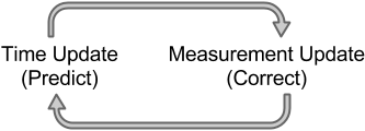
The Kalman Filter conditions recursively the current estimate on all of the past measurements. The time update projects the current state estimate ahead in time, while the measurement update adjusts the projected estimate by an actual measure at that time. Kalman Filter Algorithm
Generally, statistical notation will note an a priori estimation with a “super minus” symbol next to the variable, so for our case the a priori estimations for the state and the covariance are noted as $$\mathbf{\hat{x}^{-}}$$ and $$\mathbf{\hat{P}^{-}}$$, respectively. For the a posteriori estimations we do not use any special symbol, we merely don’t use the “super minus”.
The time-stamps are represented in discrete time usually with a sub-index $$k$$ starting from zero (initial state). Knowing this, in order to use the Kalman filter we always have to specify the initial priors for the state and covariance.
In the probabilistic approach, we define the Expected Value $$\mathbf{E}[\mathbf{x_0}]$$ and Covariance $$\mathbf{Cov}[\mathbf{x_0}]$$ as the initial state and initial covariance, respectively. In practice we can start with simpler values:
$$\mathbf{\hat{x}_0} = \begin{pmatrix} 0 & 0 & 0 \end{pmatrix}^T$$
$$\mathbf{\hat{P}_0} = \begin{pmatrix} 1 & 0 & 0 \ 0 & 1 & 0 \ 0 & 0 & 1 \end{pmatrix}$$
Note that the covariance matrix is a squared matrix, whose dimensions correspond to the length of the state vector. Initially we can set this a priori covariance matrix as the identity, which means that every state is directly correlated to itself. Further estimations will update this matrix to a better fit for every element.
The simplest form of the Kalman Filter process can be resumed as:
Time Update
- Project the a priori State.
$$\mathbf{\hat{x}^-}k = \mathbf{A} \mathbf{\hat{x}}{k-1}$$
{:start=“2”} 2. Project the a priori Covariance.
$$\mathbf{\hat{P}^-}k = \mathbf{A} \mathbf{\hat{P}^-}{k-1} \mathbf{A}^T+ \mathbf{Q}$$
Measurement Update
{:start=“3”} 3. Estimate the Measurement prediction covariance.
$$\mathbf{S}k = \mathbf{H} \mathbf{\hat{P}^-}{k} \mathbf{H}^T+ \mathbf{R}$$
{:start=“4”} 4. Compute the Kalman Gain.
$$\mathbf{K}k = \mathbf{\hat{P}^-}{k} \mathbf{H}^T \mathbf{S^{-1}}k = \mathbf{\hat{P}^-}{k} \mathbf{H}^T \big(\mathbf{H} \mathbf{\hat{P}^-}_{k} \mathbf{H}^T+ \mathbf{R}\big)^{-1}$$
This is a long equation, I know, but a simpler way to see it is as the ratio explained above:
$$\mathbf{K}k = \frac{\mathbf{\hat{P}^-}{k} \mathbf{H}^T}{\mathbf{S}k} = \frac{\mathbf{\hat{P}^-}{k} \mathbf{H}^T}{\mathbf{H} \mathbf{\hat{P}^-}_{k} \mathbf{H}^T+ \mathbf{R}}$$
NOTE: Don’t dare to show the latter notation to a Mathematician or you will be yelled at.
{:start=“5”} 5. Compute the innovation.
$$\mathbf{r}_k = \mathbf{z}k - \mathbf{H} \mathbf{\hat{x}^-}{k}$$
{:start=“6”} 6. Update the State estimate (a posteriori state).
$$\mathbf{\hat{x}}_k = \mathbf{\hat{x}^-}_k + \mathbf{K}_k \mathbf{r}_k = \mathbf{\hat{x}^-}_k + \mathbf{K}_k \big(\mathbf{z}k - \mathbf{H} \mathbf{\hat{x}^-}{k}\big)$$
{:start=“7”} 7. Update the Covariance (a posteriori covariance).
$$\mathbf{\hat{P}}_k = \mathbf{\hat{P}^-}_k - \mathbf{K}_k\mathbf{S}_k\mathbf{K}_k^T$$
Other literature computes this Covariance with:
$$\mathbf{\hat{P}}_k = \big(\mathbf{I}-\mathbf{K}_k\mathbf{H}\big)\mathbf{\hat{P}^-}_k$$
Both are equivalent and return the same result. Hypothetically, the second version requires less operations (added in the transpose of the first), but I haven’t personally checked this. You’re welcome to do so.
Among the wide range of formulae, we observe that there are four elements remaining constant throughout the whole process:
- $$\mathbf{A}$$ = Transition Matrix. This matrix performs all linear operations between the previous state $$\mathbf{\hat{x}^-}_{k-1}$$ and the current a priori state $$\mathbf{\hat{x}^-}_k$$.
- $$\mathbf{Q}$$ = Process Noise Covariance Matrix. Defines the dynamic disturbance noise of out physical model calculations.
- $$\mathbf{R}$$ = Measurement Noise Covariance Matrix. Reflects the distribution of the noise in the measurements.
- $$\mathbf{H}$$ = Observation Matrix. Relates the measured values with the calculated values.
Its implementation in an M-file script (for MATLAB or Octave) is reduced to a few lines of code:
% Predict
xhat = A*xhat;
P    = A*P*A' + Q;
% Correct
S    = H*P*H' + R;
K    = P*H'/S;
r    = z - H*xhat;
xhat = xhat + K*r;
P    = P - K*SK';
In Python we can equally simplify it in a function:
import numpy as np
import scipy.linalg as lin

def kf(xhat, P, z, A, Q, R, H):
    # Initial parameters
    m = len(xhat)
    n = len(z)
    I = np.eye(m)
    # KF - Prediction
    xhat = np.dot(A, xhat)
    P    = np.dot(A, np.dot(P, A.T)) + Q
    # KF - Update
    S    = np.dot(H, np.dot(P, H.T)) + R
    K    = np.dot(P, np.dot(H.T, lin.inv(S)))
    v    = z.reshape((n,1)) - np.dot(H, xhat)
    xhat = xhat + np.dot(K, v)
    P    = np.dot((I - np.dot(K, H)), P)
    return xhat, P
Let us see, how our robot accurately estimates its position using a Kalman Filter in every step:
| Estimation | Representation |
|---|---|
| $$\mathbf{\hat{x}^-}k = \mathbf{A} \mathbf{\hat{x}}{k-1}$$ |  |
| $$\mathbf{\hat{P}^-}k = \mathbf{A} \mathbf{\hat{P}^-}{k-1} \mathbf{A}^T+ \mathbf{Q}$$ |  |
| $$\mathbf{R}$$, $$\mathbf{z}_k$$ |  |
| $$\mathbf{K}k = \mathbf{\hat{P}^-}{k} \mathbf{H}^T \big(\mathbf{H} \mathbf{\hat{P}^-}_{k} \mathbf{H}^T+ \mathbf{R}\big)^{-1}$$ |  |
| $$\mathbf{\hat{x}}_k = \mathbf{\hat{x}^-}_k + \mathbf{K}_k \big(\mathbf{z}_k - \mathbf{H} \mathbf{\hat{x}^-}_k\big)$$ |  |
| $$\mathbf{\hat{P}}_k = \mathbf{\hat{P}^-}_k - \mathbf{K}_k\mathbf{S}_k\mathbf{K}_k^T$$ |  |
| Start Again | 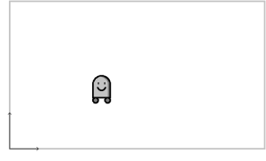 |
Model Parameters
The selection of the constant matrices $$\mathbf{A}$$, $$\mathbf{Q}$$, $$\mathbf{R}$$ and $$\mathbf{H}$$ define the behaviour of our filtering. These matrices specify how our data will be handled, and the secret of our estimations lies inside them.
The structure of the transition matrix $$\mathbf{A}$$ depends directly on the linear predictions and on the number of elements in the state vector.
The observation matrix $$\mathbf{H}$$ depends on the number of elements in $$\mathbf{\hat{x}}_k$$ as well, but also on the number of sensors to be used.
Of our interest now are the matrices $$\mathbf{Q}$$ and $$\mathbf{R}$$, the noise covariances. The Measurement noise covariance $$\mathbf{R}$$ specifies the deviation of the sensor measurements. The easiest way to build it is by giving the parameters provided in the datasheet of the sensors.
If the datasheet of the wheel encoders in our robot specify that they have a tolerance of $$\pm 3%$$, its standard deviation will be noted by $$\sigma_r^2=0.03$$. Using two wheel encoders (for X- and Y-axis), the resulting Measurement Noise Covariance $$\mathbf{R}$$ is:
$$\mathbf{R} = \begin{pmatrix}\sigma_r^2 & 0 \ 0 & \sigma_r^2\end{pmatrix} = \begin{pmatrix}0.03 & 0 \ 0 & 0.03\end{pmatrix}$$
The size of $$\mathbf{R}$$ is determined by the number of sensors to be used.
In the other hand, the Process Noise Covariance Matrix $$\mathbf{Q}$$ indicating how “reliable” our mathematical model cannot be so easily estimated. For that we have to go back to our characterization of the model.
In our models, the Transition Matrix $$\mathbf{A}$$ will perform the desired linear operations that compute the a priori estimated state, as represented in the first step of the KF. This is called typically the Process Model.
The formal solution for the distributions in a Process Model is given by recursive Bayesian filtering equations, which relate the behaviour of our models in a time-invariant domain (sampling frequency is assumed constant.)
Thanks to this recursive relation in time, the model can also be equivalently expressed in continuous-time state equations as:
$$\frac{d\mathbf{x}(t)}{dt} = \mathbf{Fx}(t) + \mathbf{Lw}(t)$$
$$\mathbf{F}$$ and $$\mathbf{L}$$ are constant matrices, which characterize the changes of the Process model. Notice that we introduce these two new terms for the construction of the model.
This might be difficult to grasp initially, but don’t put too much attention to it if you go into practice. The model above basically describes the behaviour of the changes in our Process model. Understand only that.
We have defined our Process Model as a series of linear time-invariant operations:
$$\mathbf{\hat{x}^-}k = \mathbf{A} \mathbf{\hat{x}}{k-1}$$
$$\mathbf{\hat{P}^-}k = \mathbf{A} \mathbf{\hat{P}^-}{k-1} \mathbf{A}^T+ \mathbf{Q}$$
And the model with the linear operations over $$\mathbf{F}$$ and $$\mathbf{L}$$ describes the changes in it, including the process noise $$\mathbf{w}$$ with power spectral density $$\mathbf{q}$$.
The relation between these matrices can be used to estimate the Process Noise Covariance $$\mathbf{Q}$$ that we need. And that’s the only reason I presented them here.
To get the discretized matrix $$\mathbf{Q}$$ you calculate it as:
$$\mathbf{Q} = \int_{0}^{\Delta t_k} \big(e^{\mathbf{F}(\Delta t_k-\tau)}\big) \mathbf{LqL}^T \big(e^{\mathbf{F}(\Delta t_k-\tau)}\big)^T d\tau$$
where $$\Delta t_k = t_k - t_{k-1}$$ is the step-size of the discretization. Boom!
For simpler cases, the calculation of $$\mathbf{Q}$$ can be made analytically, but attempting a step-wise calculation of $$\mathbf{Q}$$ can easily lead to mistakes that are hard to identify. That’s why I don’t recommend you to do it (unless you feel like a Hierophant of Maths. In that case do it and please share your results :D).
The linearity of the model allows us to perform an easy and fast computation of $$\mathbf{Q}$$ by simply applying the basic operations given in the formula above, using the following matrix fraction decomposition:
$$\mathbf{\Phi} = \begin{pmatrix}\mathbf{F} & \mathbf{LqL}^T \ \mathbf{0} & -\mathbf{F}^T \end{pmatrix}$$
$$\begin{pmatrix}\mathbf{C} \ \mathbf{D}\end{pmatrix} = e^{(\mathbf{\Phi}\Delta t)}\begin{pmatrix}\mathbf{0} \ \mathbf{I}\end{pmatrix}$$
These two submatrices are used to build the Process Noise Covariance Matrix $$\mathbf{Q}$$, which is finally computed as
$$\mathbf{Q}=\mathbf{C}\mathbf{D}^{-1}$$
Notice that the Design Matrix $$\mathbf{\Phi}$$ is twice as big as the Model Matrix $$\mathbf{F}$$. For example, if $$\mathbf{F}$$ is a $$3\times 3$$ matrix, then $$\mathbf{\Phi}$$ will be a $$6\times 6$$ matrix.
This would not severely slow down the process, because it is computed only once at the beginning of the filtering and assumed constant afterwards.
The simplified set of operations to obtain $$\mathbf{Q}$$ is reduced to the following lines of an M-File
% Q := Process Noise Covariance
m   = length(xhat);
q   = 0.01;
L   = eye(size(F,1));
Phi = [F L*q*L'; zeros(m) -F'];
CD  = expm(Phi*dt) * [zeros(m);eye(m)];
Q   = CD(1:m,:)/CD((m+1):(2*m),:);
or in Python:
import numpy as np
import scipy.linalg as lin

def buildQ(qc,F,dt):
    m   = len(qc)
    Qc  = np.eye(m)*qc
    Phi = np.vstack((np.hstack((F, Qc)),np.hstack((np.zeros((m,m)),-F.T))))
    CD  = np.dot(lin.expm(np.dot(Phi,dt)),np.vstack((np.zeros((m,m)),np.eye(m))))
    Q   = lin.solve(CD[m::,:],CD[0:m,:])
    return Q
Important observations should be made here. First about the code: the most unusual function here is expm, which simply performs the matrix exponential.
This function is found in almost every mathematical library of any major programming languages. Be aware that it does not perform an element-wise exponential power of the matrix.
>> A = [1        1        0
        0        0        2
        0        0       -1];
>> expm(A)
ans =
   2.7183   1.7183        1.0862
   0        1.0000        1.2642
   0             0        0.3679
A second observation to make is about the value behind the spectral density $$\mathbf{q}$$ of the white noise.
Unfortunately, we have no way to identify it automatically, and we must set it manually to a defined value. In the code above it is equal to $$0.01$$ (smaller variances in our mathematical model), but feel free to observe its influence on the system when it is changed.
This spectral density can be also estimated as a vector with the same length as the state vector $$\mathbf{\hat{x}}$$, whose values match with those of the state vector. So that they will be also compared independently against each other.
Take the model of the robot again. We have specified that we will use accelerometers to track its position. So, when predicting the values ahead in the Process Model, the resulting values for the a priori state must update as:
$$\mathbf{\hat{x}}k^- \leftarrow \mathbf{\hat{x}}{k-1}^- + \mathbf{\hat{\dot{x}}}{k-1}^-\Delta t + \frac{1}{2}\mathbf{\hat{\ddot{x}}}{k-1}^-\Delta t^2$$
$$\mathbf{\hat{\dot{x}}}{k}^- \leftarrow \mathbf{\hat{\dot{x}}}{k-1}^- + \mathbf{\hat{\ddot{x}}}_{k-1}^-\Delta t$$
$$\mathbf{\hat{\ddot{x}}}{k}^- \leftarrow \mathbf{\hat{\ddot{x}}}{k-1}^-$$
In that case the Transition matrix $$\mathbf{A}$$ would look like:
$$\mathbf{A} = \begin{pmatrix}1 & \Delta t & \frac{1}{2}\Delta t^2 \ 0 & 1 & \Delta t \ 0 & 0 & 1\end{pmatrix}$$
Because:
$$\underbrace{\begin{pmatrix}\hat{x}k \ \hat{\dot{x}}{k} \ \hat{\ddot{x}}{k}\end{pmatrix}}{\mathbf{\hat{x}}k} = \underbrace{\begin{pmatrix}1 & \Delta t & \frac{1}{2}\Delta t^2 \ 0 & 1 & \Delta t \ 0 & 0 & 1\end{pmatrix}}{\mathbf{A}} \underbrace{\begin{pmatrix}\hat{x}{k-1} \ \hat{\dot{x}}{k-1} \ \hat{\ddot{x}}{k-1}\end{pmatrix}}{\mathbf{\hat{x}}_{k-1}}$$
The corresponding Model Matrix $$\mathbf{F}$$ of this system is then:
$$\mathbf{F} = \begin{pmatrix}0 & 1 & \Delta t \ 0 & 0 & 1 \ 0 & 0 & 0\end{pmatrix}$$
It is not a coincidence if you spot a similarity between $$\mathbf{A}$$ and $$\mathbf{F}$$. As mentioned before, $$\mathbf{F}$$ describes the behaviour of the differential (the changes) of the state $$\mathbf{x}$$. It would be natural to think that it is also related to the transition between states. And it is! It turns out that they are can be described as:
$$\mathbf{A} = e^{(\mathbf{F}\Delta t)}$$
Thanks to this relation we can get the transition matrix $$\mathbf{A}$$ by computing the matrix exponential of $$\mathbf{F}$$ and the sampling value $$\Delta t$$.
A = expm(F*dt);
and in Python:
A = lin.expm(np.dot(F,dt))
Yes! One line of code will produce the entire Transition Matrix $$\mathbf{A}$$ that will govern all linear operations in our system. But I would suggest you to build $$\mathbf{A}$$ manually for a better precision.
This is why it is important to define $$\mathbf{F}$$, because through this matrix we can quickly compute the two important matrices $$\mathbf{A}$$ and $$\mathbf{Q}$$.
Extended Kalman Filter
The magic of Kalman filtering is possible thanks to the ability we have to handle our data with simple additions and multiplications. They are performed in large vectors and matrices but are still simple linear operations.
Life is not so simple in reality, and that is one big limitation of the Kalman Filter: it only works as a linear process.
Most systems work in a nonlinear space, and we know that since we try to integrate angular displacements with the simple linear translations, which leads us to a series of nonlinear functions to update the state.
This might sound bad and we could try to throw everything to the ground, but before sadness invades our minds we can consider the KF again.
As said, the KF works in a linear space and needs linear inputs so it will return linear outputs. The Extended Kalman Filter (EKF) solves this problem by converting the nonlinear inputs into linear data around any state.
The EKF calculates the Jacobian of the a priori state and the Jacobian of its observations, so we can have the most approximate estimated state. A Jacobian is a matrix containing the derivatives of the elements of a vector with respect to a set of variables.
Redefining the model
Although the use of linearization is a demanding task, the steps of the Kalman filtering will not change, but only slightly its definitions and formulas, which are now governed by functions and not simple linear operations.
The system has still the state vector $$\mathbf{\hat{x}}$$ that contains the elements to estimate, but now the Process Model is defined by the nonlinear stochastic equation:
$$\mathbf{\hat{x}}k^- = f(\mathbf{\hat{x}}{k-1})$$
with a measurement estimation $$\mathbf{\hat{z}}_k$$ also defined by a nonlinear equation:
$$\mathbf{\hat{z}}_k = h(\mathbf{\hat{x}}_k^-)$$
In this case, the nonlinear function $$f$$ relates the state at the previous state step to the step at the current one, while the function $$h$$ relates the state $$\mathbf{\hat{x}}_k$$ to the measurement estimation $$\mathbf{\hat{z}}$$ (notice the difference between estimated measurement $$\mathbf{\hat{z}}$$ and the real measurement $$\mathbf{z})$$.
It is important to note that the fundamental flaw of the EKF is that the distributions are no longer normal after undergoing their respective nonlinear transformations. The EKF simply approximates the optimality of the Bayesian probability by linearization.
The EKF works almost like a regular KF iteratively predicting states ahead and correcting them with the measurements, except for $$\mathbf{A}$$ and $$\mathbf{H}$$, which vary in time based on the estimated state $$\mathbf{\hat{x}}$$ and are dependent on the function $$f$$ and the function $$h$$, respectively.
Here the Jacobian matrices enter the game and will be the strongest help by linearizing the actual state and evaluate over this linear approximations.
We want to use a linearized transition matrix $$\mathbf{A}$$ like in our normal KF and in order to get it we have to compute the Jacobian of the function $$f$$ with respect to the elements of the state vector $$\mathbf{x}$$ giving us:
$$\mathbf{A}_k = \frac{d}{d\mathbf{x}}f(\mathbf{\hat{x}}) = \begin{pmatrix}\frac{d}{dx_0}f(\hat{x}_0) & \cdots & \frac{d}{dx_j}f(\hat{x}_0) \ \vdots & \ddots & \vdots \ \frac{d}{dx_0}f(\hat{x}_j) & \cdots & \frac{d}{dx_i}f(\hat{x}_j) \end{pmatrix}$$
This Jacobian matrix $$\mathbf{A}$$ is the linearized version of the function $$f$$ defining the transition between states.
If you noticed the subscript $$k$$ in the matrix is because it will change for each timestamp, because now it depends on $$\mathbf{\hat{x}}$$.
In the same way, the nonlinear function h can be linearized and used through its Jacobian of the form:
$$\mathbf{H}_k = \frac{d}{d\mathbf{x}}h(\mathbf{\hat{x}}) = \begin{pmatrix}\frac{d}{dx_0}h(\hat{x}_0) & \cdots & \frac{d}{dx_j}h(\hat{x}_0) \ \vdots & \ddots & \vdots \ \frac{d}{dx_0}h(\hat{x}_j) & \cdots & \frac{d}{dx_i}h(\hat{x}_j) \end{pmatrix}$$
Do not be scared with such equations. They are simpler than what it seems and the only hard part is the derivation of each element if it is done manually.
You’re welcome to do so, but if you prefer to save your time (and self-embarrasment) like me I suggest you to use symbolic mathematical programs like Mathematica (or its free alternatives Maxima or SymPy), which will calculate all these elements in a fraction of a second.
Yes, now all the elements of $$\mathbf{A}$$ and $$\mathbf{H}$$ also need to be recomputed in every timestamp. The number of elements in the state vector $$\mathbf{x}$$ and the complexity of your functions $$f$$ and $$h$$ will decide the time of these computations. The EKF is then resumed as:
Time update
- Project the a priori State.
$$\mathbf{\hat{x}^-}k = f(\mathbf{\hat{x}}{k-1})$$
{:start=“2”} 2. Project the a priori Covariance.
$$\mathbf{\hat{P}^-}k = \mathbf{A} \mathbf{\hat{P}^-}{k-1} \mathbf{A}^T+ \mathbf{W}_k\mathbf{Q}\mathbf{W}_k^T$$
Measurement update
{:start=“3”} 3. Estimate the Measurement prediction covariance.
$$\mathbf{S}k = \mathbf{H} \mathbf{\hat{P}^-}{k} \mathbf{H}^T+ \mathbf{V}_k\mathbf{R}\mathbf{V}_k^T$$
{:start=“4”} 4. Compute the Kalman Gain.
$$\mathbf{K}k = \mathbf{\hat{P}^-}{k} \mathbf{H}^T \mathbf{S^{-1}}k = \mathbf{\hat{P}^-}{k} \mathbf{H}^T \big(\mathbf{H} \mathbf{\hat{P}^-}_{k} \mathbf{H}^T+ \mathbf{V}_k\mathbf{R}\mathbf{V}_k^T\big)^{-1}$$
{:start=“5”} 5. Compute the innovation.
$$\mathbf{r}_k = \mathbf{z}k - h( \mathbf{\hat{x}^-}{k})$$
{:start=“6”} 6. Update the State estimate (a posteriori state).
$$\mathbf{\hat{x}}_k = \mathbf{\hat{x}^-}_k + \mathbf{K}_k \mathbf{r}_k = \mathbf{\hat{x}^-}_k + \mathbf{K}_k \big(\mathbf{z}k - h( \mathbf{\hat{x}^-}{k})\big)$$
{:start=“7”} 7. Update the Covariance (a posteriori covariance).
$$\mathbf{\hat{P}}_k = \mathbf{\hat{P}^-}_k - \mathbf{K}_k\mathbf{S}_k\mathbf{K}_k^T$$
Or, again, with:
$$\mathbf{\hat{P}}_k = \big(\mathbf{I}-\mathbf{K}_k\mathbf{H}\big)\mathbf{\hat{P}^-}_k$$
What the hell are matrices $$\mathbf{W}$$ and $$\mathbf{V}$$?
Fear not, my friend! Those are the Jacobian matrices of the functions $$f$$ and $$h$$ with respect to the process noise $$w$$ and measurement noise $$v$$, respectively:
$$\mathbf{W}=\frac{d}{dw}f(\mathbf{\hat{x}})$$
$$\mathbf{V}=\frac{d}{dv}h(\mathbf{\hat{x}})$$
As mentioned before, the values for the gaussian noises are unknown in reality, but we can use the covariances $$\mathbf{Q}$$ and $$\mathbf{R}$$ in a similar way as in the standard Kalman filter by defining $$\mathbf{W}$$ and $$\mathbf{V}$$ as identities.
Kaboom! Now you have the basic tools to go out and play with KFs. I know it is not easy to get, but re-read the points you don’t get, go to other documentation to confirm, and, most important, apply what you see.
Any questions? Suggestions? What should I explain more?
Great References
- An Introduction to the Kalman Filter; Greg Welch, Gary Bishop; SIGGRAPH 2001.
- Optimal Filtering with Kalman Filters and Smoothers, a Manual for the Matlab toolbox EKF/UKF; version 1.3; Jouni Hartikainen, Arno Solin, and Simo Särkkä.
- Sensor Fusion using the Kalman Filter; Katharina Buckl; CAMPAR TUM; 2005.